What you're really asking about is less to do with Astronomy and more to do with mathematics. You're basically asking if, given a system of differential equations, will a unique solution exist for all time? For an answer, you should check out the Existence and Uniqueness theorems of differential equations. You'd be better to ask questions like this on the Mathematics stack exchange.
However, to discuss the particular, astronomical case you've asked about, the answer is yes, you can run that system both forwards and backwards if you know some initial state. Newtonian mechanics is completely deterministic in that if you know all the equations of motion involved, as well as the entire state of the system at a given time, you can figure out the state of that system at any other time, both in the past and the future.
To speak to your particular 3-body orbiting problem though, I'll say that the system of equations is not solvable in closed form - that is, you can't write down an analytic solution to the equations like you could for the 2-body case. As userLTK states, you can write down approximate solutions in the restricted 3-body problem, where one mass is significantly less than the other two and orbits under specific conditions.
To get a solution at any time $\hat{t}$, you need to use numerical methods. Of course numerical methods are inherently flawed. Numerical errors build up the longer you simulate due to time steps which are not infinitesimal, from errors within the numerical algorithms used, and general floating point errors. In theory, if you had a computer with infinite precision and infinite computing power, you could solve a 3-body (or n-body) system perfectly, but we live in the real world where such things are impossible.
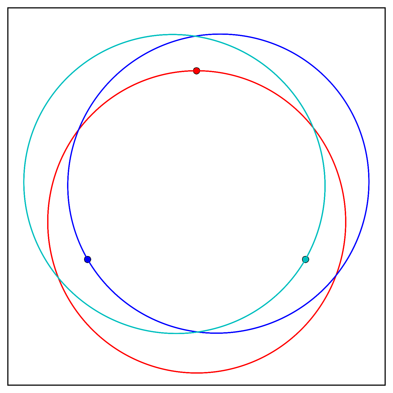
To prove though, that you can figure out the state at any time in the past or present for a three body body, I've written a basic simulation in Python 3. It can run both forwards and backwards from a given start condition and start time. Essentially it puts three nearly identical masses in contrived starting positions and velocities. Below the code are plots of results.
import numpy as np
from numpy.linalg import norm
from matplotlib.pyplot import *
from time import time

# Define physical constants
G = 6.67408E-11          # Gravitational Constant, m^3 kg^-1 s^-2

# Define body 1 parameters
m1 = 2.2E30                # Mass, kg
x1 = np.array([0,1E11])  # Position, m
v1 = np.array([-3.5E4,0])  # Velocity, m/s

# Define body 2 parameters
m2 = 1.9E30
x2 = np.array([1E11*np.cos(210*np.pi/180),
               1E11*np.sin(210*np.pi/180)])
v2 = np.array([3E4*np.cos(300*np.pi/180),
               3E4*np.sin(300*np.pi/180)])

# Define body 3 parameters
m3 = 2E30
x3 = np.array([1E11*np.cos(330*np.pi/180),
               1E11*np.sin(330*np.pi/180)])
v3 = np.array([3E4*np.cos(60*np.pi/180),
               3E4*np.sin(60*np.pi/180)])

# Define simulation parameters
n = 3                    # Number of bodies, unitless
t = 0                    # Simulation time, s
dt = 1E4                 # Simulation time step, s
tEnd = 1E8               # Simulation end time, s
m = np.array((m1,m2,m3)) # All masses
x = np.vstack((x1,x2,x3))# All positions
v = np.vstack((v1,v2,v3))# All velocities
xHist = [[list(x1)],[list(x2)],[list(x3)]]
vHist = [[list(v1)],[list(v2)],[list(v3)]]

# Simulate until end time is reached
start = time()
while True:
    # Calculate acceleration
    a = []
    for i in range(n):
        a.append(0)
        for j in range(n):
            if i == j: continue
            a[-1] += - G * m[j] / norm(x[i]-x[j])**3 * (x[i] - x[j])

    # Update velocities
    for i,vi,ai in zip(range(n),v,a):
        vi += ai * dt
        vHist[i].append(list(vi))

    # Update positions
    for i,xi,vi in zip(range(n),x,v):
        xi += vi * dt
        xHist[i].append(list(xi))

    # Update time and end simulation if past tEnd
    t += dt
    if dt > 0 and t > tEnd: break
    if dt < 0 and t < tEnd: break

end = time()
print('Simulation finished in {:.4f} seconds.'.format(end-start))

# Convert xHist and vHist to np arrays
xHist = np.array(xHist)
vHist = np.array(vHist)

# Plot everything up
figure()
for i,c in enumerate(['or','ob','oc']):
    # Plot starting positions
    plot(xHist[i,0,0], xHist[i,0,1], c)
for i,c in enumerate(['-r','-b','-c']):
    # Plot path of star
    plot(xHist[i,:,0], xHist[i,:,1], c)
gca().set_aspect(1)
gca().set_xticks([])
gca().set_yticks([])
show(block = False)
Note, the plots show the initial positions of the stars as the points and then trace out their paths over time.
Path of three masses for $t<t_0$
 In this scenario, the three masses end up in the contrived scenario. I ran the simulation backwards by setting the timestep
 dt and the end time tEnd to be negative.
Path of three masses for $t_0<t$
 From here, the simulation is run forwards with positive
 dt and tEnd, starting from the same contrived scenario as above.
Note how chaotic and unstable this system is. The entire system only remains a 3-body system for less than 6 years. Before that the three masses are separate and doing their own thing. They "coincidentally" meet (because I set it up so they should), orbit around each other for a little less than 6 years, and one gets ejected, resulting in the other two continuing to orbit one another.
Contrived Scenario with $m_1=m_2=m_3$, $|v_1|=|v_2|=|v_3|$, and all positions $120^o$ from each other
 Just for fun, a "stable" 3-body problem with all stars of equal mass and orbits. This is really an unstable equilibrium orbit and any perturbations will screw it up and you'll see what you saw in the above two graphs. In fact, if you run this long enough, the numerical instabilities of my code will result in the orbits breaking down. This numerical instability, as I said above, is inherent in any numerical solution and cannot be overcome, only minimized. I find that, using the numerical method I did, my system is resistant to numerical instabilities for about 7 years. If I want to run this any longer (and continue to be accurate), I need more robust numerical methods.


