Partial answer:
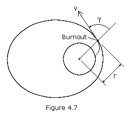
What Braeunig calls gamma or zenith angle is actually beta!
...and γ is the angle between the position and the velocity vectors, called the zenith angle (see Figure 4.7))

According to @TomSpilker's answer
This is a problem that has plagued groups of people very knowledgeable about orbital dynamics but who learned using different textbooks: there are two different definitions of "flight path angle"!!
In addition to $\gamma$, the angle between the tangential direction and the velocity vector, there is $\beta$, the angle between the radial direction and the velocity vector. People often say "flight path angle" without saying which definition they're using. Confusing! (I just noticed that the diagram in Julio's answer also shows $\beta$)
If you work with $\beta$ instead of $\gamma$, $\beta$ is given by
$$\arccos\left(\frac{\mathbf{r \centerdot v}}{|\mathbf{r}| \ |\mathbf{v}|} \right) \tag{1} $$
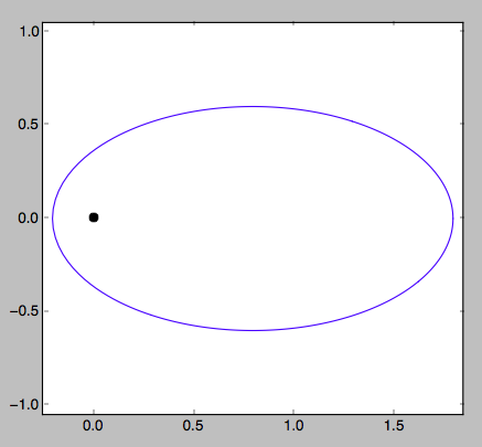
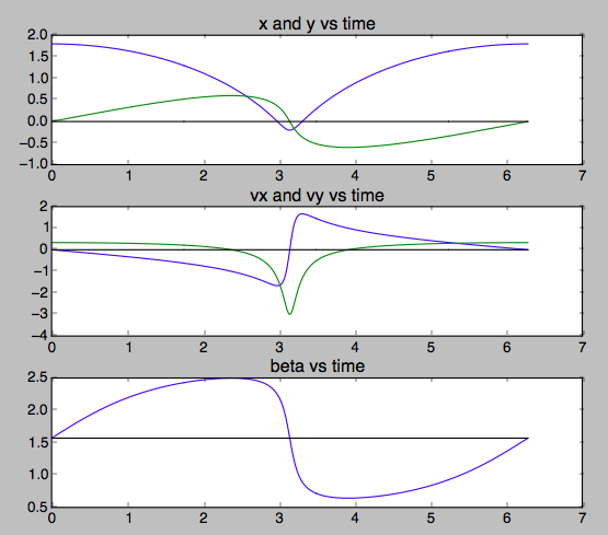
So Braeunig's gamma is NASA's beta. It's positive from peri to apo, and negative from apo to peri. Because I'm not smart enough to do it with math, I'll do it with Python.
I'm doing this in dimensionless units, so the period is 2π and the semi-major axis is unity. You can see beta's behavior over one orbit, positive moving towards apoapsis, then negative moving towards periapsis.


def deriv (X, t):
    x, v = X.reshape(2, -1)
    acc = -x * ((x**2).sum())**-1.5
    return np.hstack((v, acc))

import numpy as np
import matplotlib.pyplot as plt
from scipy.integrate import odeint as ODEint

halfpi, pi, twopi = [f*np.pi for f in (0.5, 1, 2)]
degs, rads = 180/pi, pi/180

time = np.linspace(0, twopi, 361)

r0 = 1.8
v0 = np.sqrt(2./r0 - 1)  # vis-viva

X0 = np.hstack([r0, 0, 0, v0])

answer, info = ODEint(deriv, X0, time, full_output=True)

x,    v      = answer.T.reshape(2, 2, -1)
rn = x/np.sqrt((x**2).sum(axis=0))
vn = v/np.sqrt((v**2).sum(axis=0))

x, y, vx, vy = answer.T

beta = np.arccos((rn*vn).sum(axis=0))

if True:
    plt.figure()
    plt.plot(x, y)
    plt.plot([0], [0], 'ok', markersize=8)
    x0, y0 = 0.5*(x.min() + x.max()), 0.5*(y.min() + y.max())
    hwx, hwy = (np.abs(x-x0)).max(), (np.abs(y-y0)).max()
    hw = 1.05*max(hwx, hwy)
    plt.xlim(x0-hw, x0+hw)
    plt.ylim(y0-hw, y0+hw)
    plt.show()

if True:
    plt.figure()
    plt.subplot(3, 1, 1)
    plt.plot(time, x)
    plt.plot(time, y)
    plt.plot(time, np.zeros_like(time), '-k')
    plt.title('x and y vs time')
    plt.subplot(3, 1, 2)
    plt.plot(time, vx)
    plt.plot(time, vy)
    plt.plot(time, np.zeros_like(time), '-k')
    plt.title('vx and vy vs time')
    plt.subplot(3, 1, 3)
    plt.plot(time, beta)
    plt.plot(time, halfpi*np.ones_like(time), '-k')
    plt.title('beta vs time')
    plt.show()
