4
$\begingroup$

What is the error range for calculations for the time of 1st-4th contacts for a given GPS coordinate on Earth?

I observed through a telescope the 3rd and 4th contacts and compared against SkySafari and Stellarium. I found SkySafari showed contacts about 10 seconds earlier for the same location vs Stellarium. Stellarium was very close to my measurements for 3rd contact (1-2 seconds). To get the calculation I zoomed the GUI and tweaked the time until it was closest to the contact. Estimates for 4th contact (transit end) are much harder to visually time.

This got me interested to know if there is a gold standard for such calculations, and what is the range of error for it. For forecasts n years out is the error range n times more?

Stellarium Web visual calculation of 3rd contact time

$\endgroup$
3
  • 1
    $\begingroup$ NASA would be the gold standard, but jpl.nasa.gov/edu/events/2019/11/11/… doesn't provide timing down to the second. You could try naif.jpl.nasa.gov/naif/webgeocalc.html (or CSPICE, the library on which this page is based) to get down-to-the-second transit times. $\endgroup$
    – user21
    Commented Nov 13, 2019 at 15:36
  • $\begingroup$ @barrycarter I tried wgc.jpl.nasa.gov:8443/webgeocalc/#OccultationFinder but couldn't figure it out. For kernel selection I picked "Solar System Kernels" for lack of a better guess, and picked ellipsoid shapes for mercury and sun. I got CSPICE_N0066: CSPICE.gfoclt: SPICE(INVALIDFRAME): [gfoclt_c --> GFOCLT --> GFOCCE --> ZZGFOCIN] Supposed body-fixed frame ITRF93 for front target 199 is actually centered on body 399. So it's clearly not meant for amateurs like myself. However, I see there are some tutorials (naif.jpl.nasa.gov/naif/tutorials.html) which may explain things. $\endgroup$
    – Automaton
    Commented Nov 13, 2019 at 21:56
  • $\begingroup$ Hmm, it worked for me and gave me "2019-11-11 12:35:26.990156 UTC" for start time and "2019-11-11 18:04:14.482772 UTC" for end time. I'll screenshot my settings in just a sec $\endgroup$
    – user21
    Commented Nov 13, 2019 at 23:09

2 Answers 2

3
$\begingroup$

This got me interested to know if there is a gold standard for such calculations

For the orbital mechanics and geometrical aspects, the NASA JPL Development Ephemerides are commonly used. These have errors for the Sun and inner planets of tens of kilometers or less.

...and what is the range of error for it. For forecasts n years out is the error range n times more?

That depends on the specific ephemeris you use and a lot of other details. The ephemerides are build from a huge body of observations and calculations and it's not a simple thing to say. I think the errors will be dominated by the definition of the edge of the Sun for several decades or even centuries. Farther out in time, the ephemeris itself will have some error that may increase with time in either direction.

Below I calculate that the apparent radial speed at which mercury crosses the "edge" of the Sun's disk is about -70.6 and +70.6 km/sec, assuming a "radius" of 695,700 km, using the Python package Skyfield which in turn uses the NASA JPL Development Ephemerides. For this calculation I used DE421.

I used Caracas as the location since the whole event was visible from this location. The main calculation happens in these three lines. The .observe() method automatically does the light-time correction for the positions.

sun_astrometric     = caracas.at(times).observe(sun) 
mercury_astrometric = caracas.at(times).observe(mercury)
angular_separation  = sun_astrometric.separation_from(mercury_astrometric).radians

I put the words "edge" and "radius" in quotes earlier because these are not well defined for things like stars and gas giant planets. There are definitions that can be used to define nominals for these, in the case of the Sun it's when the opacity reaches 2/3 or something like that.

70 km is a pretty small distance at the edge of the Sun. From this answer you can see that there is a region of a few hundred kilometers where things are changing. It's hard to say exactly what defines the "edge" of the Sun in order to say when the hard edge of rocky Mercury will be seen to touch it. I can't be sure, but I have a hunch that you can get several seconds of ambiguity based on how the edge of the Sun is defined.

Wikipedia even lists **two different values for the radius that differ by 642 km*!* At 70 km/sec that's almost ten seconds right there!

Equatorial radius   
  695,700 km  [7]
  696,342 km  [8]

From this answer:

From Chapter 2: The Photosphere of Timo Nieminen's thesis Solar Line Asymmetries: Modelling the Effect of Granulation on the Solar Spectrum
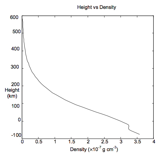
density versus hight above the Sun's surface

density and other parameters versus hight above the Sun's surface

Figure 2-3: The Holweger-Müller Model Atmosphere

7 Holweger, H. and Müller, E. A. “The Photospheric Barium Spectrum: Solar Abundance and Collision Broadening of Ba II Lines by Hydrogen”, Solar Physics 39, pg 19-30 (1974). Extra points have been cubic spline interpolated by J. E. Ross. The optical properties (such as the optical depth and the opacity) of a model atmosphere are, obviously, very important, and will be considered later. See table C-4 for complete details of the Holweger-Müller model atmosphere including all depth points used.

8The height scale is not arbitrary. The base of the photosphere (height = 0 km) is chosen to be at standard optical depth of one (i.e. 𝜏 5000Å = 1 ).

approximate transit of Venus 11-11-2019 from Caracas

Python script using the Skyfield package to calculate some things about the 11-Nov-2019 transit of Mercury across the Sun as seen from the city of Caracas, Venezuela.

import numpy as np
import matplotlib.pyplot as plt
from skyfield.api import Topos, Loader

# https://astronomy.stackexchange.com/questions/33918/accuracy-of-mercury-transit-calculations

load        = Loader('~/Documents/fishing/SkyData')  # avoids multiple copies of large files
data        = load('de421.bsp')
ts          = load.timescale()
bodies      = ('sun', 'mercury', 'earth')

seconds               = 12*3600. + np.arange(0, 390*60+1, 10)
hours                 = seconds/3600.
times                 = ts.utc(2019, 11, 11, hours)

sun,  mercury, earth  = [data[x] for x in bodies]
caracas               = earth + Topos(latitude_degrees  = 10.48,
                                      longitude_degrees = -66.90,
                                      elevation_m = 900.)

sun_astrometric     = caracas.at(times).observe(sun) 
mercury_astrometric = caracas.at(times).observe(mercury)
angular_separation  = sun_astrometric.separation_from(mercury_astrometric).radians
distance_to_sun     = sun_astrometric.distance().km
distance            = distance_to_sun * np.tan(angular_separation)
r_sun               = 695700*np.ones_like(hours)
thing               = distance < r_sun
i_in                = np.argmax(thing)
thing[:i_in+1]      = True
i_out               = np.argmax(~thing)
hours_in, hours_out = hours[[i_in, i_out]]

dt                  = seconds[1] - seconds[0]
ddistance_dt        = (distance[1:] - distance[:-1])/dt

if True:
    plt.figure()
    fs = 12
    plt.subplot(2, 1, 1)
    plt.plot(hours, distance)
    plt.plot(hours[[i_in, i_out]], distance[[i_in, i_out]], 'ok')
    plt.plot(hours, r_sun, '-k')
    plt.ylim(0, None)
    plt.title('projected distance from Sun center (km,)', fontsize=fs)
    plt.subplot(2, 1, 2)
    plt.plot(hours[:-1], ddistance_dt)
    plt.plot(hours[[i_in, i_out]], ddistance_dt[[i_in, i_out]], 'ok')
    plt.xlabel('hours UTC 2019-11-11', fontsize=fs)
    plt.title('d projected distance/dt (km/s)', fontsize=fs)
    print(ddistance_dt[[i_in, i_out]])
    plt.show()
$\endgroup$
5
  • 1
    $\begingroup$ The reference to the JPL model is useful. Point taken that "edge" is not clearly defined for the sun. Mm $\endgroup$
    – Automaton
    Commented Nov 16, 2019 at 0:32
  • $\begingroup$ @Automaton This isn't an exhaustive list of uncertainties at all, but I think it is the largest one. Uncertainties in the positions of the Sun, Mercury and Earth are much smaller in comparison. See for example ssd.jpl.nasa.gov/pub/eph/planets/ioms/de423.iom.pdf and also This orientation is the limiting error source for the orbits of the terrestrial planets, and corresponds to orbit uncertainties of a few hundred meters. for example for DE431. $\endgroup$
    – uhoh
    Commented Nov 16, 2019 at 2:19
  • 1
    $\begingroup$ and also Uncertainties in the JPL Planetary Ephemeris $\endgroup$
    – uhoh
    Commented Nov 16, 2019 at 2:23
  • 1
    $\begingroup$ The graphs in Uncertainties in the JPL Planetary Ephemeris are very interesting. I'm familiar with the N body physics problem which is characterised as chaotic, so I was expecting uncertainties rapidly go up with time e.g. exponentially but it isn't the case in these graphs. $\endgroup$
    – Automaton
    Commented Nov 28, 2019 at 2:34
  • $\begingroup$ @Automaton orbits in the solar system are definitely chaotic, but it becomes a problem over millions of years or more, way beyond where these ephemerides are calculated. There is tightly constrained and accurate enough observational data over enough time now to predict with fairly good accuracy over tens of thousands of years. As a random example, see the arXiv paper linked in this answer and search for "chaotic". $\endgroup$
    – uhoh
    Commented Nov 28, 2019 at 3:27
1
$\begingroup$

This is not an answer.

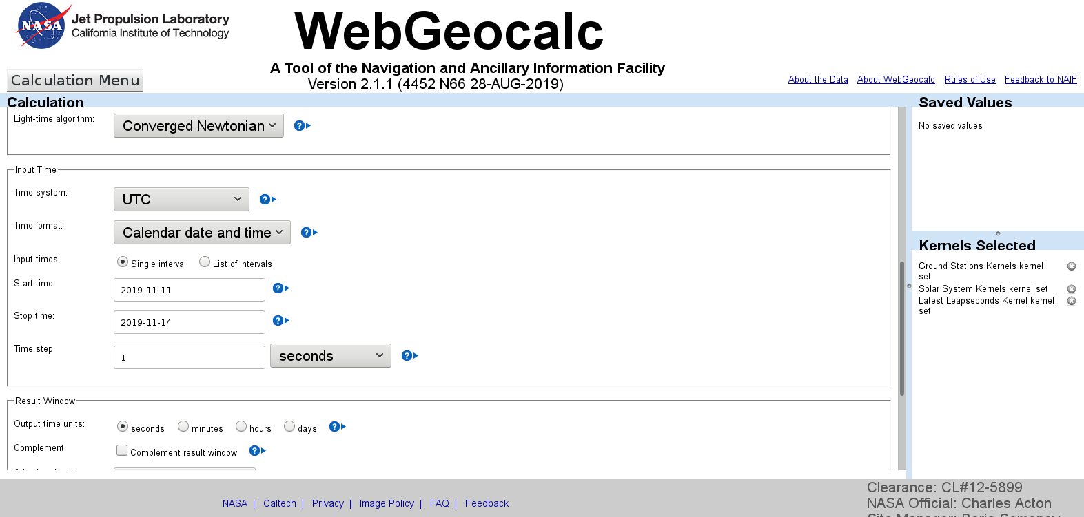
Settings I used:

enter image description here

enter image description here

enter image description here

Results I got:

enter image description here enter image description here enter image description here

The kernel "pds/wgc/mk/latest_lsk_v0004.tm" was also used, but got clipped in the very last screenshot (it would be at the very bottom of the screenshot)

EDIT: As you note in the comments, "EARTH" means the Earth's geocenter. If you click on the help down arrow, it says

`SPICE name or numeric ID of a body, whether built-in or defined in loaded kernels. Examples:

input MRO or -74 for Mars Reconnaissance Orbiter;
input JUPITER or 599 for the Jupiter center of mass;
input JUPITER_BARYCENTER or 5 for the Jupiter system barycenter;
input DSS-63 or 399063 for the DSN station numbered 63.`

While there are several pages that talk about DSNs (such as http://www-pi.physics.uiowa.edu/docs/spice/NAIF_IDS.HTML under "Ground Stations" and https://deepspace.jpl.nasa.gov/about/ which mentions the first 4 stations [the only four that have actual names]), I couldn't find a list of positions except for the first 4.

The closest I could get is https://naif.jpl.nasa.gov/pub/naif/generic_kernels/spk/stations/a_old_versions/dsnstns.cmt which shows the xyz positions of the stations from which you could presumably calculate latitude and longitude and find the station closest to you.

At some point, though, it'd be easier just to use CSPICE directly.

$\endgroup$
2
  • $\begingroup$ I was able to replicate this. The issue I had was I entered ITRF93 as a guess for body frame. Now I see the results are extremely precise into fractions of a second, and it doesn't resolve both the inner and outer contact points for the transit. As you noted clearly, there isn't an error range or standard deviation, so it would be good to hear back if someone is aware of a calculator that provides that as well. Another limitation here is this app doesn't account for where on earth the observation is (I suppose it considers earth's center point, given no entry field for GPS coordinates). $\endgroup$
    – Automaton
    Commented Nov 14, 2019 at 1:40
  • 1
    $\begingroup$ I edited to note you can get observations from certain points on Earth. $\endgroup$
    – user21
    Commented Nov 14, 2019 at 2:46

You must log in to answer this question.

Not the answer you're looking for? Browse other questions tagged .