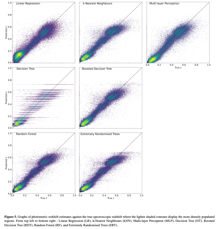
The banding is an inherent consequence of the way simple decision trees work. Each leaf in such decision trees provides a leaf-specific answer, right or wrong. In this case, each leaf in the decision tree provides a specific red shift ($z$) value.
To illustrate, I'll start with a zero-branch decision tree. Regardless of the input photometric data, this zero-branch decision tree will give the same answer. This singular answer will be $\bar z$, the average of all of the true red shift values in the training data set. (Note: The authors chose mean square error as the metric used in the decision tree. The mean is the value that minimizes the mean square error.) When plotted as a predicted $z$ versus true $z$ scatter plot when applied against the test data set, the result will be a single horizontal band at that training data set $\bar z$ value.
The above is ludicrously over the top, but it illustrates why a decision tree will show bands in a predicted versus true scatter plot. With a single branch decision tree there will be two leaves in the tree, one for the then branch of the single decision and another for the else branch, and thus two bands in the scatter plot. A two-branch decision tree will have three leaves (so three bands), and so on. One can sometimes count the number of leaves in a decision tree simply by counting the number of bands in the scatter plot.
