Return to Revisions

This is a partial answer.

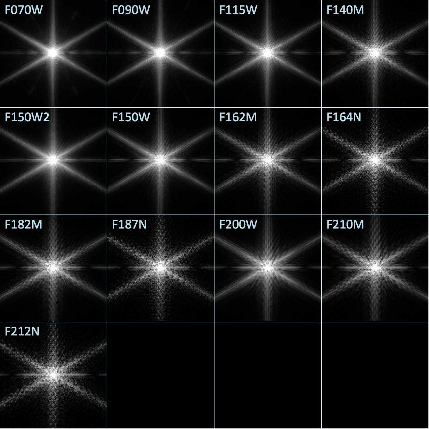
Each small mirror will impose its own strong six-spiked diffraction pattern in the telescopes point-spread function. For telescope apertures build from a large number of hexagonal mirrors this will dominate the point-spread function.

The choice of pattern for the tiling of small mirrors to fill the full aperture will have a much smaller effect.

JWST simulated point spread function from James Webb Space Telescope User Documentation's NIRCam Point Spread Functions

I found an analytical expression for the diffraction pattern from (or at least the Fourier transform of) a single hexagonal aperture (or flat mirror) in this answer to How does Fraunhofer diffraction depend on the orientation of the sides of a lens? in Physics SE.

Hexagonal aperture. I take the following function: $$ \begin{split} h(x,y) = \left[\theta(2y+\sqrt{3})-\theta(2y-\sqrt{3})\right]\cdot \left[\theta(y-\sqrt{3}(x-1))-\theta(y-\sqrt{3}(x+1))\right]\cdot\\ \left[\theta(y-\sqrt{3}(-x-1))-\theta(y-\sqrt{3}(1-x))\right] \end{split}$$ With $\theta(x)$ -- is a [Heaviside step function][2].
While it is in principle possible to calculate the Fourier transform of this by hand, I've just fed it to CAS and I've got something like this: $$\frac{2\sqrt{3}\omega_x\left(\cos\frac{\omega_x}{2}\cos\frac{\sqrt{3}\omega_y}{2} -\cos\omega_x\right)-6\omega_y\sin\frac{\omega_x}{2}\sin\frac{\sqrt{3}\omega_y}{2}} {\pi \omega_x(\omega_x^2-3\omega_y^2)}$$ ...plus some singular terms that I've dropped.
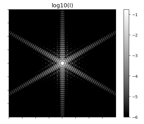
Plotting square of the result (from -100 to 100)

Here's my plot and a python script based on that expression:

import numpy as np
import matplotlib.pyplot as plt

def hexamp(omx, omy):
    """diffraction amplitude hexagonal aperture from
    https://physics.stackexchange.com/a/9910/83380"""
    C, S = np.cos, np.sin
    rt3 = np.sqrt(3)
    
    term_1 = 2 * rt3 * omx * (C(omx/2.)*C(rt3*omy/2.) - C(omx))
    
    term_2 = -6 * omy * S(omx/2.) * S(rt3*omy/2.)

    bottom = np.pi * omx * (omx**2 - 3.*omy**2)

    return (term_1 + term_2)/bottom

omega = np.arange(-100, 100, 0.1)
omx, omy = np.meshgrid(omega, omega)

amplitude = hexamp(omx, omy)

I = np.abs(amplitude)**2

if True:
    plt.figure()
    plt.imshow(np.log10(I), cmap='gray', vmin=-6)
    plt.gca().set_aspect('equal')
    plt.gca().axes.xaxis.set_ticklabels([])
    plt.gca().axes.yaxis.set_ticklabels([])
    plt.colorbar()
    plt.title('log10(I)', fontsize=14)
    plt.show()