It is well known that diffraction resolution of a telescope depends on the exterior radius of aperture: One can, for instance, use just a narrow outer ring of a parabolic mirror and the resolution will be the same as it were the whole mirror (obviously, intensity will be much much smaller)
The premise of your question is false. I tried to convince you to separate it out as a separate question, but to no avail. So I'll answer it here instead.
From comment:
I personally made computation of the telescope transfer function for annular aperture and found that support of the function in the fourier space is the same as for circular aperture. This is an elementary excercise.
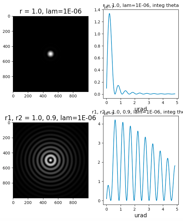
To help illustrate that a narrow annular aperture has much worse resolution than the full aperture, I'll do a quick comparison. The first plot is the diffraction pattern (scale is +/- 0.5 arcseconds) for a clear aperture of 2 million wavelengths (e.g. 1 meter radius with 1 micron wavelength), and the second is for the same aperture with a 0.9 meter obstruction.
I use Airy disks and Babinet's principle to subtract the E-field of the obstruction before squaring. For this symmetry there's no need to do an explicit Fourier analysis, the Airy disk is the Fourier transform of the circular aperture step function. (see also)
This is for an annulus with outer radius 1.0 and inner 0.9. If it was 1.0 and 0.99 it would look much much worse!
Now, take such a ring telescope, say, 3cm wide ring which is 100 meters in diameter.
That would give you a giant splat pattern of roughly the same size as a simple 3 cm diameter telescope would.

Python script:
from scipy.special import j1
import matplotlib.pyplot as plt
import numpy as np

def get_E(a, lam, theta):
    ka  = (twopi/lam) * a
    x   = ka * np.sin(theta)
    return a * (2. * j1(x) / x)

halfpi, pi, twopi = [f*np.pi for f in (0.5, 1, 2)]
degs, rads        = 180/pi, pi/180

arcsecs = np.arange(0, 0.5, 0.0001)[1:]
theta   = (arcsecs/3600.) * rads

r1, r2  = 1.0, 0.9
lam     = 1E-06

arcsecs   = np.linspace(-1, 1, 1000) # arcsec (skips zero to avoid singularity)
Xas, Yas, = np.meshgrid(arcsecs, arcsecs)
Ras       = np.sqrt(Xas**2 + Yas**2)
theta     = Ras * pi / 3600. / 180.

E1, E2    = [sign*get_E(r, lam, theta) for r, sign in ((r1, +1), (r2, -1))]
asec      = np.linspace(0, 1.0, 500)[1:]
th        = asec * pi / 3600. / 180.
e1, e2    = [sign*get_E(r, lam, th) for r, sign in ((r1, +1), (r2, -1))]

Etot = E1 + E2
etot = e1 + e2

if True:
    plt.figure()
    plt.subplot(2, 2, 1)
    plt.imshow(E1**2, cmap='gray')
    plt.title('r = 1.0, lam=1E-06', fontsize=16)
    plt.subplot(2, 2, 3)
    plt.imshow(Etot**2, cmap='gray')
    plt.title ('r1, r2 = 1.0, 0.9, lam=1E-06', fontsize=16)
    plt.subplot(2, 2, 2)
    plt.plot(1E+06*th, th*e1**2) # weight by th for azimuthal (phi) integration
    plt.xlabel('urad', fontsize=14)
    plt.title('r = 1.0, lam=1E-06, integ theta')
    plt.subplot(2, 2, 4)
    plt.plot(1E+06*th, th*etot**2) # weight by th for azimuthal (phi) integration
    plt.title('r1, r2 = 1.0, 0.9, lam=1E-06, integ theta')
    plt.xlabel('urad', fontsize=14)
    plt.show()
