Here is what I did:
- Based on their masses, it is safest to initially consider Jupiter and Saturn as well as Uranus. It might also be fruitful to include the Earth in the analysis, to get relative positions, observation angles, etc. So, I will be considering:
- Sun
- Earth
- Jupiter
- Saturn
- Uranus
- Neptune
- Get the standard gravitational parameters (μ) for all of them
- Get initial positions and velocities via JPL/HORIZONS for all these planets. I had some data lying around from J2000.5, so I just used the state vectors from the 1st of January, 2000, at noon.
- Write an N-body integrator with built-in MATLAB tools. Integrate this incomplete Solar system once without Neptune, and once with Neptune included.
- Analyze and compare!
So, here's my data, and N-body integrator:
function [t, yout_noNeptune, yout_withNeptune] = discover_Neptune()

    % Time of integration (in years)
    tspan = [0 97] * 365.25 * 86400;

    % std. gravitational parameters [km/s²/kg]
    mus_noNeptune = [1.32712439940e11; % Sun
                     398600.4415       % Earth
                     1.26686534e8      % Jupiter
                     3.7931187e7       % Saturn
                     5.793939e6];      % Uranus

    mus_withNeptune = [mus_noNeptune
                       6.836529e6]; % Neptune

    % Initial positions [km] and velocities [km/s] on 2000/Jan/1, 00:00
    % These positions describe the barycenter of the associated system,
    % e.g., sJupiter equals the statevector of the Jovian system barycenter.
    % Coordinates are expressed in ICRF, Solar system barycenter
    sSun     = [0 0 0 0 0 0].';
    sEarth   = [-2.519628815461580E+07  1.449304809540383E+08 -6.175201582312584E+02,...
                -2.984033716426881E+01 -5.204660244783900E+00  6.043671763866776E-05].';
    sJupiter = [ 5.989286428194381E+08  4.390950273441353E+08 -1.523283183395675E+07,...
                -7.900977458946710E+00  1.116263478937066E+01  1.306377465321731E-01].';
    sSaturn  = [ 9.587405702749230E+08  9.825345942920649E+08 -5.522129405702555E+07,...
                -7.429660072417541E+00  6.738335806405299E+00  1.781138895399632E-01].';
    sUranus  = [ 2.158728913593440E+09 -2.054869688179662E+09 -3.562250313222718E+07,...
                 4.637622471852293E+00  4.627114800383241E+00 -4.290473194118749E-02].';
    sNeptune = [ 2.514787652167830E+09 -3.738894534538290E+09  1.904284739289832E+07,...
                 4.466005624145428E+00  3.075618250100339E+00 -1.666451179600835E-01].';

    y0_noNeptune   = [sSun; sEarth; sJupiter; sSaturn; sUranus];
    y0_withNeptune = [y0_noNeptune; sNeptune];

    % Integrate the partial Solar system
    % once with Neptune, and once without
    options = odeset('AbsTol', 1e-8,...
                     'RelTol', 1e-10);

    [t, yout_noNeptune]   = ode113(@(t,y) odefcn(t,y,mus_noNeptune)  , tspan, y0_noNeptune  , options);
    [~, yout_withNeptune] = ode113(@(t,y) odefcn(t,y,mus_withNeptune),     t, y0_withNeptune, options);

end

% The differential equation
%
%    dy/dt = d/dt [r₀ v₀ r₁ v₁ r₂ v₂ ... rₙ vₙ]
%          = [v₀ a₀ v₁ a₁ v₂ a₂ ... vₙ aₙ]
%
%  with
%
%    aₓ = Σₘ -G·mₘ/|rₘ-rₓ|² · (rₘ-rₓ) / |rₘ-rₓ|
%       = Σₘ -μₘ·(rₘ-rₓ)/|rₘ-rₓ|³
%
function dydt = odefcn(~, y, mus)

    % Split up position and velocity
    rs = y([1:6:end; 2:6:end; 3:6:end]);
    vs = y([4:6:end; 5:6:end; 6:6:end]);

     % Number of celestial bodies
    N = size(rs,2);

    % Compute interplanetary distances to the power -3/2
    df  = bsxfun(@minus, permute(rs, [1 3 2]), rs);
    D32 = permute(sum(df.^2), [3 2 1]).^(-3/2);
    D32(1:N+1:end) = 0; % (remove infs)

    % Compute all accelerations
    as = -bsxfun(@times, mus.', D32);              % (magnitudes)
    as = bsxfun(@times, df, permute(as, [3 2 1])); % (directions)
    as = reshape(sum(as,2), [],1);                 % (total)

    % Output derivatives of the state vectors
    dydt = y;
    dydt([1:6:end; 2:6:end; 3:6:end]) = vs;
    dydt([4:6:end; 5:6:end; 6:6:end]) = as;

end
Here is the driver script I used to get some nice plots out:
clc
close all

% Get coordinates from N-body simulation
[t, yout_noNeptune, yout_withNeptune] = discover_Neptune();

% For plot titles etc.
bodies = {'Sun'
          'Earth'
          'Jupiter'
          'Saturn'
          'Uranus'
          'Neptune'};


% Extract positions
rs_noNeptune   = yout_noNeptune  (:, [1:6:end; 2:6:end; 3:6:end]);
rs_withNeptune = yout_withNeptune(:, [1:6:end; 2:6:end; 3:6:end]);


% Figure of the whole Solar sysetm, just to check
% whether everything went OK
figure, clf, hold on
for ii = 1:numel(bodies)
    plot3(rs_withNeptune(:,3*(ii-1)+1),...
          rs_withNeptune(:,3*(ii-1)+2),...
          rs_withNeptune(:,3*(ii-1)+3),...
          'color', rand(1,3));
end

axis equal
legend(bodies);
xlabel('X [km]');
ylabel('Y [km]');
title('Just the Solar system, nothing to see here');


% Compare positions of Uranus with and without Neptune
rs_Uranus_noNeptune   = rs_noNeptune  (:, 13:15);
rs_Uranus_withNeptune = rs_withNeptune(:, 13:15);

figure, clf, hold on

plot3(rs_Uranus_noNeptune(:,1),...
      rs_Uranus_noNeptune(:,2),...
      rs_Uranus_noNeptune(:,3),...
      'b.');

plot3(rs_Uranus_withNeptune(:,1),...
      rs_Uranus_withNeptune(:,2),...
      rs_Uranus_withNeptune(:,3),...
      'r.');

axis equal
xlabel('X [km]');
ylabel('Y [km]');
legend('Uranus, no Neptune',...
       'Uranus, with Neptune');


% Norm of the difference over time
figure, clf, hold on

rescaled_t = t/365.25/86400;

dx = sqrt(sum((rs_Uranus_noNeptune - rs_Uranus_withNeptune).^2,2));
plot(rescaled_t,dx);
xlabel('Time [years]');
ylabel('Absolute offset [km]');
title({'Euclidian distance between'
       'the two Uranuses'});


% Angles from Earth
figure, clf, hold on

rs_Earth_noNeptune   = rs_noNeptune  (:, 4:6);
rs_Earth_withNeptune = rs_withNeptune(:, 4:6);

v0 = rs_Uranus_noNeptune   - rs_Earth_noNeptune;
v1 = rs_Uranus_withNeptune - rs_Earth_withNeptune;

nv0 = sqrt(sum(v0.^2,2));
nv1 = sqrt(sum(v1.^2,2));

dPhi = 180/pi * 3600 * acos(min(1,max(0, sum(v0.*v1,2) ./ (nv0.*nv1) )));
plot(rescaled_t, dPhi);

xlabel('Time [years]');
ylabel('Separation [arcsec]')
title({'Angular separation between the two'
       'Uranuses when observed from Earth'});
which I'll describe here step by step.
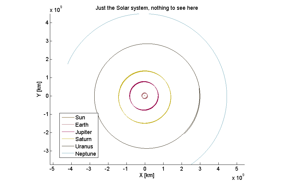
First, a plot of the Solar system to check that the N-body integrator works as it should:

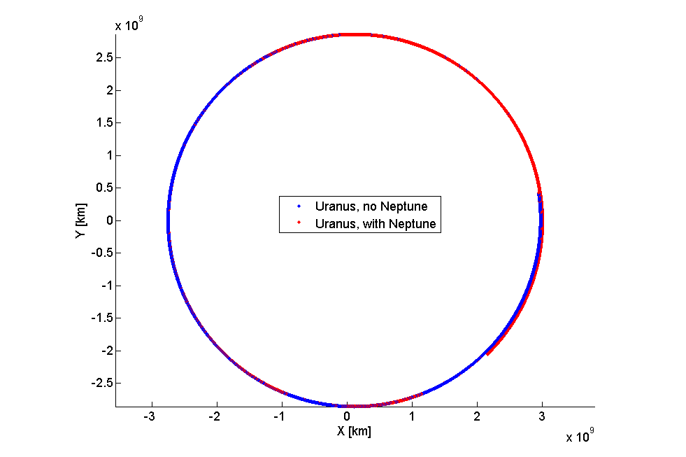
Nice! Next, I wanted to see the difference between the positions of Uranus with and without the influence of Neptune. So, I extracted just the positions of those two Uranuses, and plotted them:

...that's hardly useful. Even when zooming in greatly and rotating the heck out of it, this is just not a useful plot. So I looked at the evolution of the absolute Euclidian distance between the two Uranuses:

That's starting to look more like it! Roughly 80 years after the start of our analysis, the two Uranuses are almost 6 million km apart!
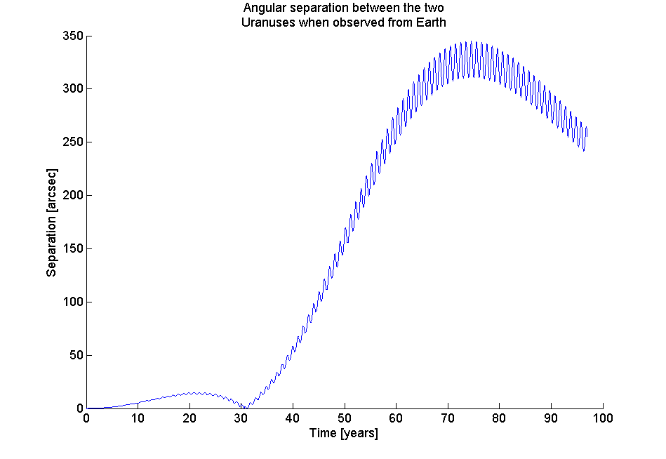
Large as that may sound, in the grander scale of things this might drown in the noise when we take measurements here on Earth. Plus, it still does not tell the whole story, as we'll see in a moment. So next, let's look at the angular difference between the observation vectors, from Earth towards the two Uranuses to see how large that angle is, and if it can stand out above the observational error thresholds:

...whoa! Well over 300 arcseconds difference, plus all sorts of wobbly bobbley timey wimey rippling going on. That seems well within the observational capabilities of the time (although I can't find a reliable source on this so quickly; anyone?)
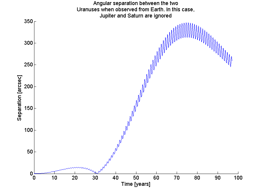
Just for good measure, I also produced that last plot leaving Jupiter and Saturn out of the picture. Although some perturbation theory had been developed in the 17th and 18th centuries, it was not very well developed and I doubt even Le Verrier took Jupiter into consideration (but again, I could be wrong; please correct me if you know more).
So, here is the last plot without Jupiter and Saturn:

Although there are differences, they are minute, and most importantly irrelevant for discovering Neptune.
