Recovering the motion of the Sun around the barycenter
The accepted answer perfectly valid, since it contains figures that closely match the data provided in JPL Horizons. In case anyone is interested, in my answer I will try to demonstrate how one can essentially reproduce this plot by actually evolving the positions and velocities of the planets in the solar system, only using:
- The vector data $(\vec{r}_i,\vec{v}_i)$ of all planets and the Sun at some initial time $t_0$.
- no specialized software - purely Python's
numpy for all calculations.
Solar Motion 1945-1995
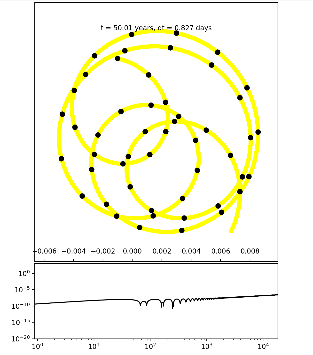
Before going into the specifics, here are the final results that I get if I use the single-day data of January 1st 1945 provided by Horizons and evolve the system for 50 years:

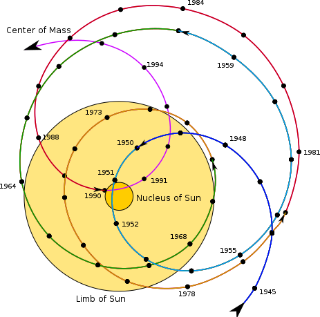
On the upper plot, the scales of the x and y axes are the equal and the units are AU. Each black dot corresponds to January 1st of a year. For comparison, the Solar radius is about 0.00465 AU. The result closely matches the figure found in Wikipedia.
The lower plot displays the evolution of the fractional energy change $\Delta E \;/\; E(t=0)$, as a function of time (in days). Since this remains substantially lower than 1, this is an indication that the evolution of the system has not gone horribly wrong.
Detailed instructions
- Download the position and velocity data from JPL Horizons. If you prefer to use their online app, select the following:
Ephemeris Type: Vector Table
Target Body: (Select Sun, Mercury, ..., Neptune iteratively)
Coordinate Center: Solar System Barycenter (SSB) [500@0]
Time Specification: Your prefered initial time, step=1 day
Table Settings: {"Output Quantities": State Vector, "Output Units": au and days, "CSV format": True}
The output with contain $[x,y,z,v_x,v_y,v_z]$ (in AU and AU/days respectively), which is all we need, along with the masses and the gravitational constant $G$.
Edit: Following the suggestion in the comments, here is a Python script that uses directly the Horizons API to get this data, by simply specifying the date ('YYYY-MM-DD'):
    import requests
    import datetime
    def get_planet_vectors(start_time_str):
        """Example usage: get_planet_vectors('2022-12-20')"""
        API_URL = 'https://ssd.jpl.nasa.gov/api/horizons.api'

        command_codes = ['10', '199', '299', '399', '499', '599', '699', '799', '899']
        options = {
            "format": 'json',
            "MAKE_EPHEM": 'YES',
            "COMMAND": None,
            "EPHEM_TYPE": 'VECTORS',
            "CENTER": '500@0',
            "START_TIME": None,
            "STOP_TIME": None,
            "STEP_SIZE": '2d',
            "VEC_TABLE": '2',
            "REF_SYSTEM": "ICRF",
            "REF_PLANE": "ECLIPTIC",
            "VEC_CORR": "NONE",
            "OUT_UNITS": 'au-d',
            "VEC_LABELS": "YES",
            "VEC_DELTA_T": "NO",
            "CSV_FORMAT": "YES",
            "OBJ_DATA": "YES",
        }

        start_time = datetime.datetime.strptime(start_time_str, '%Y-%m-%d')
        stop_time = start_time + datetime.timedelta(days=1)

        options['START_TIME'] = start_time.strftime('%Y-%m-%d')
        options['STOP_TIME'] = stop_time.strftime('%Y-%m-%d')
        planet_vectors = []
        for code in command_codes:
            options['COMMAND'] = code
            response = requests.get(API_URL, params=options)
            data = response.json()['result']
            # get the output csv data. It starts with $$SOE and ends with $$EOE
            csv_data = data[data.find('$$SOE')+5:data.find('$$EOE')-1]
            # strip any final commas and split the data into a list
            csv_data = csv_data.strip(',').split(',')
            # remove the first 2 elements, which are the time in two different formats
            csv_data = csv_data[2:]
            # convert the strings to floats
            csv_data = [float(x) for x in csv_data]
            planet_vectors.append(csv_data)
        return np.array(planet_vectors)
- Next we need a differential equation iterative solver to propagate the phase space. Note that Runge-Kutta-type solvers are not a great fit for this task, since they tend in the long-run to violate energy conservation quite severely. This resource is a contains a great introduction in accurately evolving celestial orbits. Below I have written below a 4th order symplectic integrator and a simple adaptive step-size routine, which appear to perform adequately well. Here they are:
import numpy as np
G = 0.000295912208 ## Gravitational Constant in AU^3 per Solar Masses per Days^2
class StarSystem:
    """
    Class to simulate a solar system with stars and planets
    """
    def __init__(self, phase_space=None, masses=None, n_dim=3):
        self.n_dim = n_dim
        self.step_size = 1E-3 # small initially, but adjusts automatically
        self.masses = masses
        self.phase_space = phase_space
        self.evolve = self.symplectic4

    def get_pairwise_separations(self):
        """
        Return the array of the pairwise separations of all objects in the solar system
        in the same star system.
        """
        num_objs = len(self.masses)
        positions = self.phase_space[:self.phase_space.size//2].reshape(num_objs, self.n_dim)
        # separations[i,j] is the separation vector pointing from the jth object to the ith object,
        # i.e. separations[i,j] = positions[i] - positions[j]
        separations = positions[:,np.newaxis,:] - positions[np.newaxis,:,:] # shape (num_objs, num_objs, n_dim)
        distances = np.linalg.norm(separations,axis=2) # shape (num_objs, num_objs)
        return separations, distances

    def get_accelerations(self):
        """
        Return the array of the accelerations for all objects in the star system
        """
        separations, distances = self.get_pairwise_separations()

        G_over_r3 = G/distances**3
        acceleration_components = - G_over_r3[:,:,np.newaxis] * separations * self.masses[np.newaxis,:,np.newaxis]

        accelerations = np.nansum(acceleration_components,axis=1)
        accelerations = accelerations.flatten()
        return accelerations

    def symplectic4(self, inplace=True):
        """
        Implement the symplectic integrator of 4th order to evolve
        Coefficients found in:
        http://www.slac.stanford.edu/cgi-wrap/getdoc/slac-pub-5071.pdf
        """
        h = self.step_size
        x = (2**(1/3) + 2**(-1/3) - 1)/6

        c1 = 0
        c3 = - 4*x - 1
        c2 = c4 = 2*x + 1
        d2 = d3 = -x
        d1 = d4 = x + 1/2

        c = np.array([c1,c2,c3,c4])
        d = np.array([d1,d2,d3,d4])

        original_configurations = self.phase_space.copy()

        positions, velocities = (
            self.phase_space.copy()[:self.phase_space.size//2],
            self.phase_space.copy()[self.phase_space.size//2:]
        )

        for i in range(4):
            accelerations = self.get_accelerations()
            velocities += c[i] * accelerations * h
            positions += d[i] * velocities * h
            new_phase_space = np.concatenate((positions, velocities))
            self.phase_space = new_phase_space

        if not inplace:
            # Restore the original configuration
            self.phase_space = original_configurations

        return new_phase_space

    def adapt_step(self, relError=1E-5, inplace=True):
        """
        Adapt the step size to reduce local error in positions to some specified relative error.
        """
        h = self.step_size
        ## Evolve with two steps of h
        original_configurations = self.phase_space.copy()
        self.evolve(inplace=True)
        self.evolve(inplace=True)
        positions = self.phase_space.copy()[:self.phase_space.size//2].reshape(len(self.masses), self.n_dim)

        self.phase_space = original_configurations

        ## Evolve with one step of 2*h
        self.step_size = 2*h
        self.evolve(inplace=True)
        positions2 = self.phase_space.copy()[:self.phase_space.size//2].reshape(len(self.masses), self.n_dim)
        self.phase_space = original_configurations
        self.step_size = h

        ## Calculate the maximum relative distance, defined (in 2d) as the maximum of sqrt((x1-x2)^2 + (y1-y2)^2) / sqrt(x1^2 + y1^2)
        # where (x1,y1) and (x2,y2) are the positions achieved with two steps of h and one step of 2*h
        position_differences = positions - positions2
        norm_positions = np.linalg.norm(positions, axis=1)
        norm_position_differences = np.linalg.norm(position_differences, axis=1)

        maxRelDist = np.max(norm_position_differences / norm_positions)

        # Using error estimates. Multiply by 0.85 for extra safety.
        h = 0.85 * h * (relError / maxRelDist )**(1/5)

        if inplace:
            self.step_size = h

        return h
- Evolve the system until you have reached the desired duration, e.g.
n_dim = 3
start_time_str = '1945-01-01'
duration = 50 # duration in years

masses_p = np.array([3.285E23, 4.867E24, 5.972E24, 6.39E23, 1.898E27, 5.683E26, 8.681E25, 1.024E26])
masses_p = masses_p / 1.989E30
masses = np.concatenate(([1], masses_p))

planet_vectors = get_planet_vectors(start_time_str)

# create the initial positions as an array [x1, y1, z1, x2, y2, z2, ...]
initial_positions = planet_vectors[:, :n_dim].flatten()
# create the initial velocities as an array [vx1, vy1, vz1, vx2, vy2, vz2, ...]
initial_velocities = planet_vectors[:, n_dim:].flatten()
phase_space = np.concatenate(
    (initial_positions,
    initial_velocities)
)
solar_system = StarSystem(phase_space, masses, n_dim=n_dim)
t_0 = time = 0
t_end = duration * 365.25
sun_position = []
while time<t_end:
    print(f"\r{time:.2f} days. Sun at {solar_system.phase_space[:3]} AU", end="")
    solar_system.evolve(inplace=True)
    # update your plot data using solar_system.phase_space
    time += solar_system.step_size
    sun_position.append([time, *solar_system.phase_space[:3]])
    solar_system.adapt_step(inplace=True)

data = np.array(sun_position)
time = data[:, 0]
x = data[:, 1]
y = data[:, 2]
import matplotlib.pyplot as plt
plt.plot(x, y)
plt.gca().set_aspect('equal', adjustable='box')
plt.show()


